
Lab 7
Overview
The purpose of this lab was to implement a Kalman Filter to improve the accuracy of the robot's distance measurements from the ToF sensor, therefore allowing the robot to approach a wall faster. We first defined a Python model with collected sensor data, whose values were then used as initial estimates for the actual Artemis Nano code. Kalman Filtering involves prediction and update steps, where we first predict data based on the given model model and perform an update through newly collected data to serve as another starting point. Through this lab, I learned more about Kalman filtering, specifically about the steps involved and the mathematical reasoning behind how it works.
Estimating Drag and Momentum
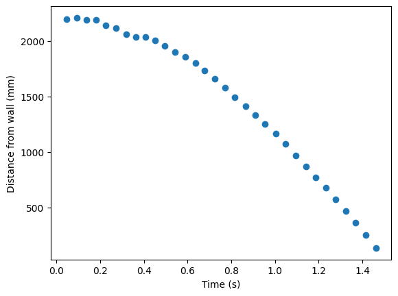
In order to estimate my robot's drag and momentum, I first gathered data from my robot's TOF sensor. I had data stored from when I did Lab 5, but I worked heavily on improving my code formatting during Lab 6, which is why I recollected my data. Furthermore, I didn't really choose to do PID when I was collecting my data, since PID would continuously change my PWM values. Instead, I set my PWM value to be 200 (my maximum possible PWM value is 220, so I went slightly lower than that). Then, when my robot was sufficiently close to the wall, I set the PWM to 0, so that the robot would stop and I wouldn't have to truncate my data. I also had to do this as my data using PID was also quite noisy. I had to experiment with this for many hours and the best data I received was the following:
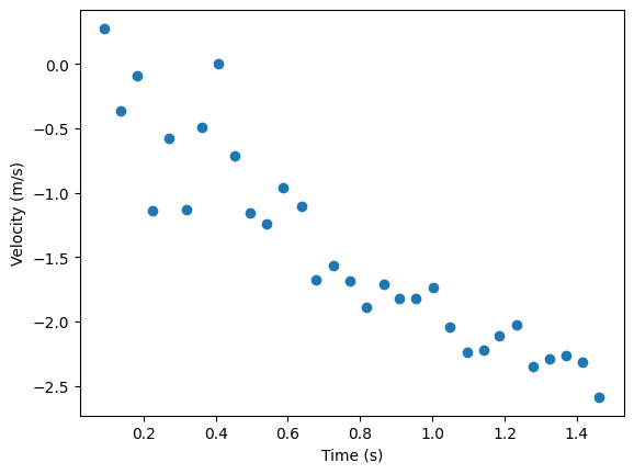
Next, I calculated the derivative of the position to get the velocity data, which I could use to calulate the rise time (time to get to the max velocity) of my robot. The derivative was calulated using a simple difference between the distance values and the time values and then dividing them: v = Δx/Δt. The resulting velocity graph is shown in Figure 2 below. One thing to note is that the velocity values are negative. This is because I used the ToF sensor raw data to calculate the velocity, in which case the recorded position decreases over time as the robot proceeds towards the wall, and therefore the change in position is negative while the change in time is positive; thus, the velocity is calculated as a negative value.
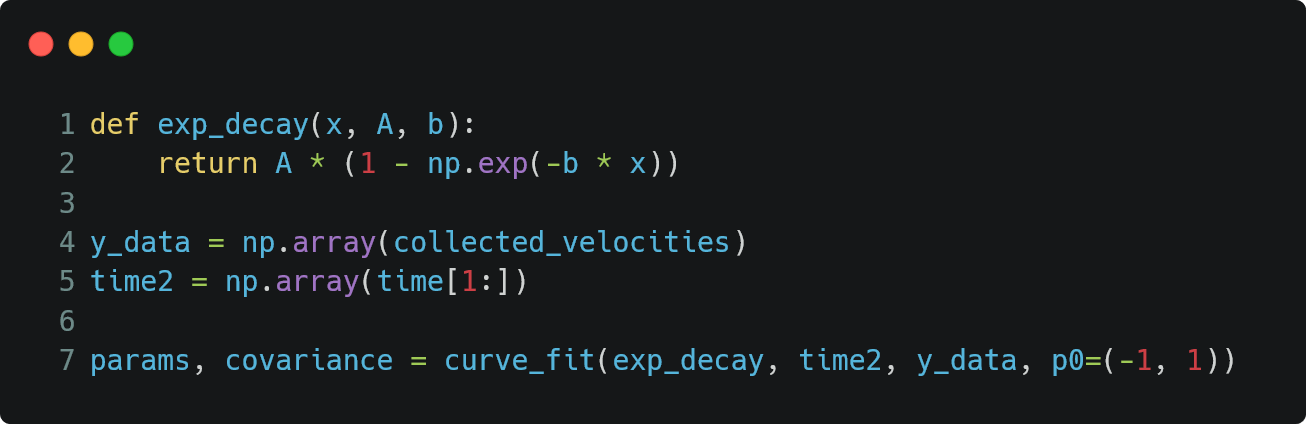
After I had collected this data, I wanted to fit an exponential decay model to my data. I chose this specific model because my robot has an physical maximum velocity that it reaches, which can be represented by the asymptote of the exponential decay model. The parameters I received for the exponential decay formula, y = A*(1-e^(-bx)), were A = -3.412 and b = 0.83.
Below is a graph of how my data was fit to an exponential curve with the parameters above. I know that the data doesn't seem to decay quite well, but I decided to stick with the data I received from this result, as I had already spent multiple hours trying to collect data and this was the best one that I had received. If the fit doesn't end up working on the Python or Arduino model, I decided that I will recollect the data.
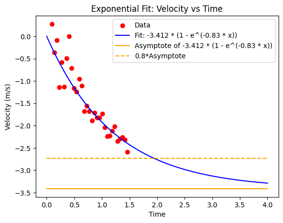
Lastly, I used the fitted parameters to calculate the 80% rise time, which was then used to calculate the drag and momentum as shown below. I used the 80% rise time and not the 100% rise time because that represents the asymptote, which the robot does not hit. Instead, I used the 80% rise time since it was closer to my collected data and was not infinite. The drag at 80% rise time can be calculated by d = 1/(velocity at 80% rise time), and the momentum at 80% rise time can be calculated by m = -d*(80% rise time)/(ln(1-80%)), where d is the drag.
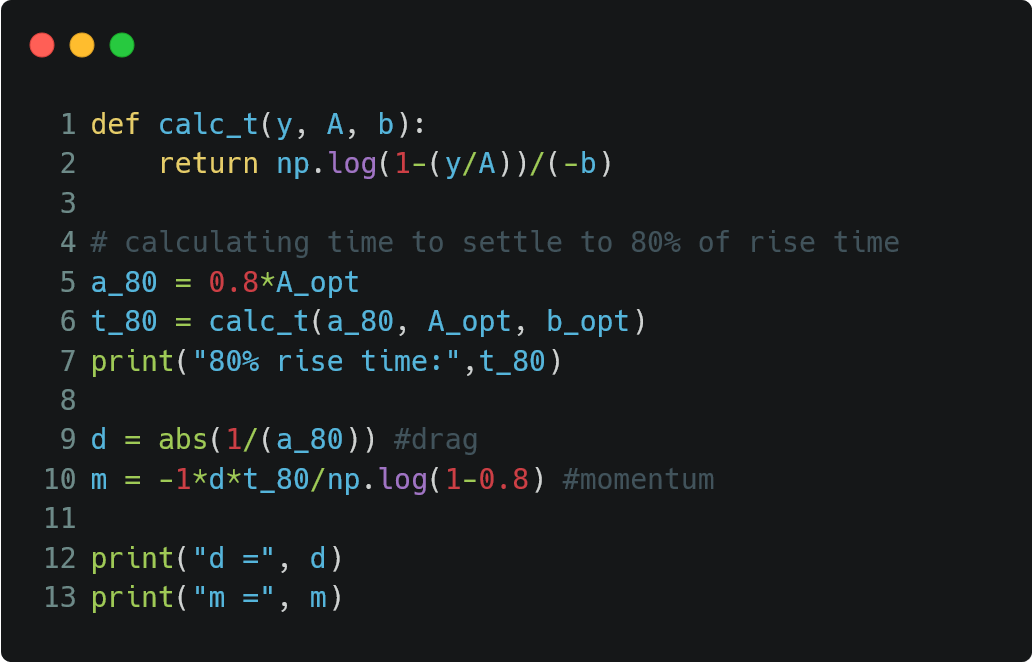
My final drag was 0.333 and momentum was 0.401.
Kalman Filtering in Python
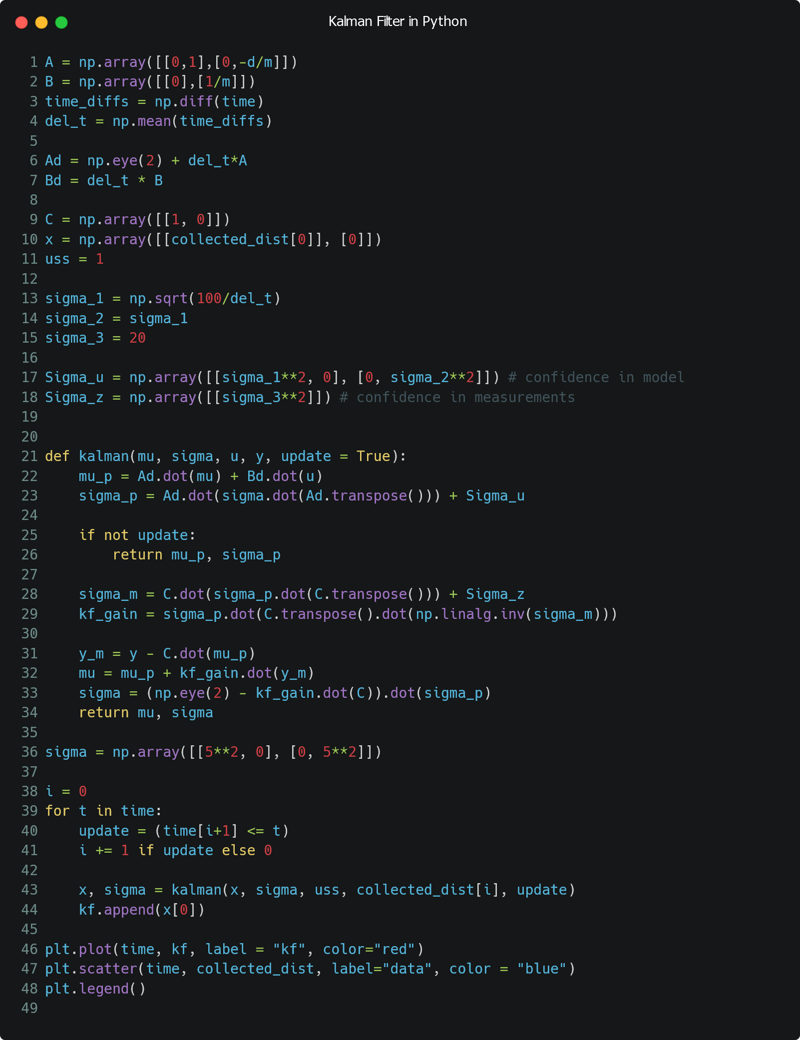
The Kalman Filter in Python was created through referencing Lecture slides and Stephan Wagner's Lab 7. Figure 6 shows the overall code for this implementation, which I will describe in further detail.
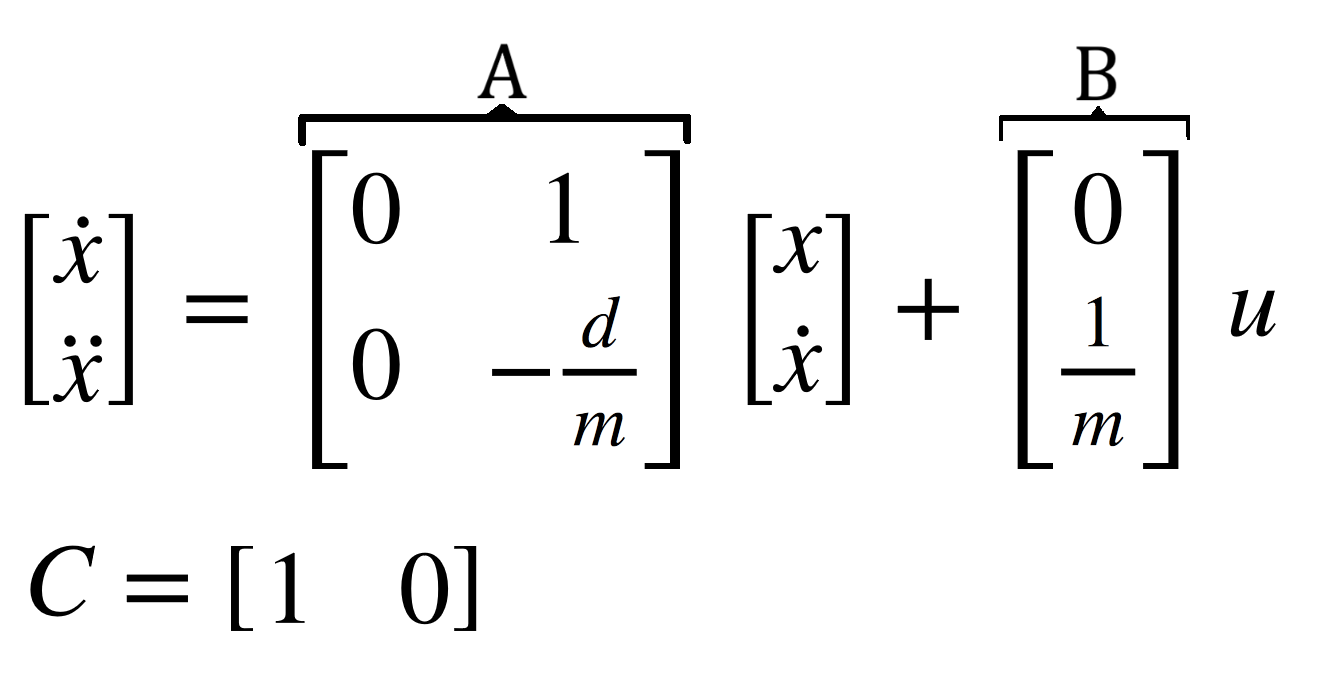
First, I combined Newton's Second Law and the relation between Force and Drag using matrices to get the equation in Figure 7 below. In my code, I set A and B as labeled in the figure, but replaced the variables with the numbers for drag and momentum which were calculated above.
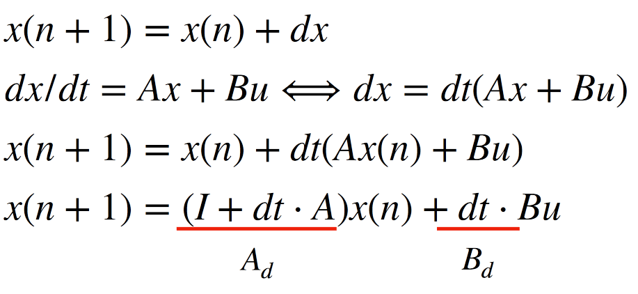
Then, I discretize the A and B matrices (called Ad and Bd, respectively) using the sample time calculated from the time data collected in the first part of this lab. The formula for doing this was derived in class and is shown in Figure 8 below (the final Ad and Bd matrices are in the last step). This essentially predicted the next position based on the previously found position data.
Next, I initialized my x matrix, which stored results for kalman filtering, to be the initial collected data. Then, I calculated my sigma (σ1, σ2, σ3, σu, σz) values similar to what I did in the python simulation, which represent the confidence in the measurements and the model. I set up my Kalman Filter function with both the update and prediction steps. Lastly, I updated my Kalman filter for every time step.
Kalman Filter on the Robot
Using the parameters calculated in the part above, I implemented the Kalman filter in Arduino. My code is quite similar to the Python code in terms of organization, except that I was handling data in real-time, instead of using stored arrays. The final code is shown in Figure 9 below.
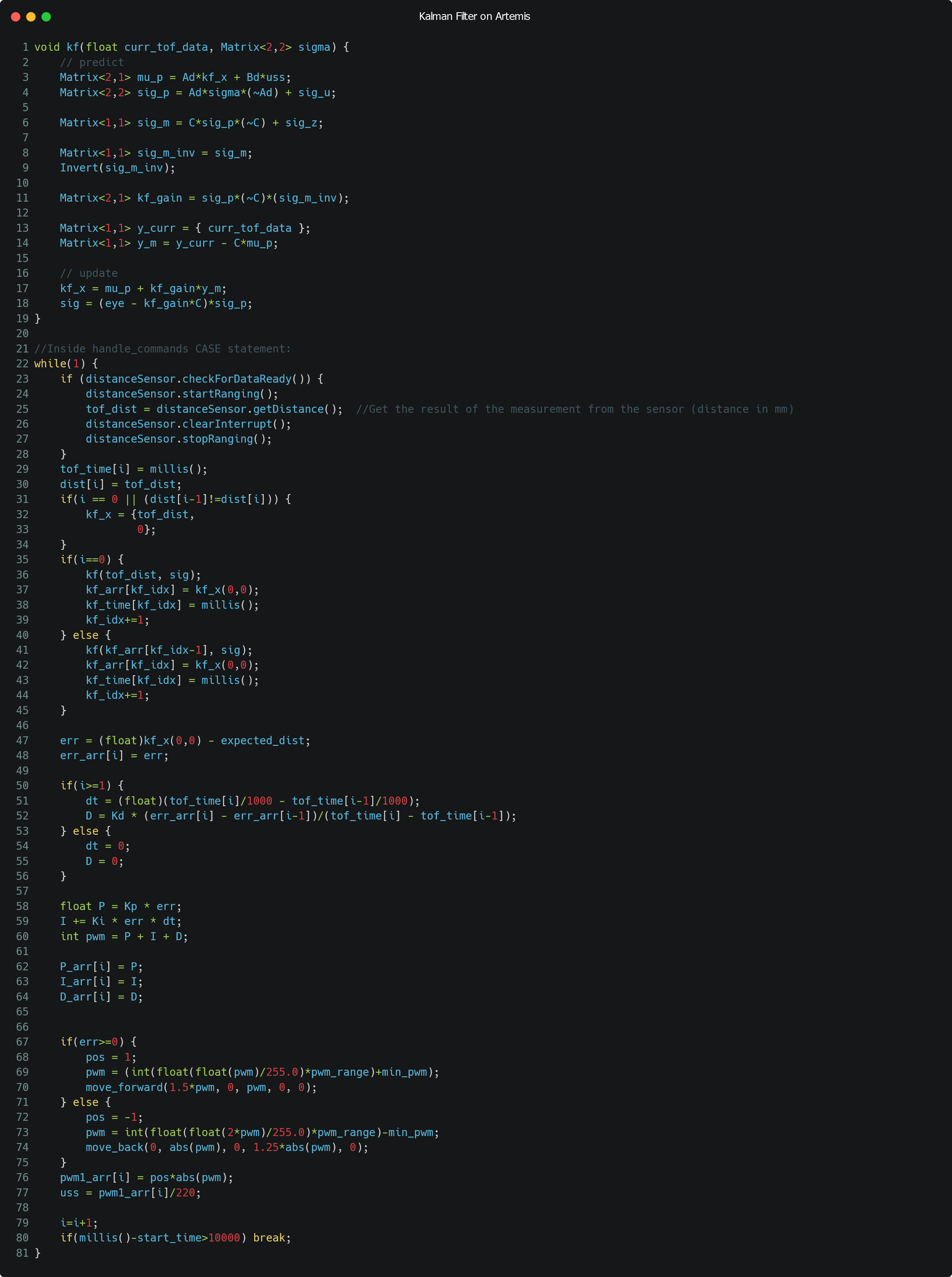
One other part that I added in this lab (as shown in the code above) was the derivative term to my PI controller to complete my PID control! The more time I spent on this robot, the more unsatisfied I became with my oscillations. Through testing, I found my Kd to be best around 1-2.
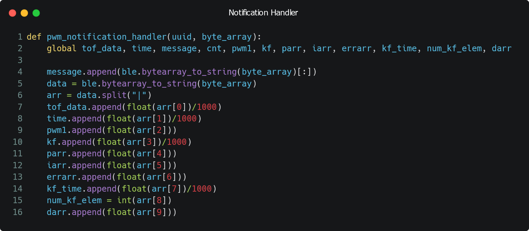
I also had to re-tune all of my PID control parameters since I was now using Kalman filter data. My Kp was around 0.07 to 0.1 and my Ki was around 0 to 0.0001. My notification handler on the Python side had a lot more parameters to store now and is shown below.
Results
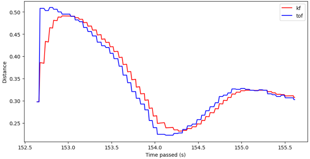
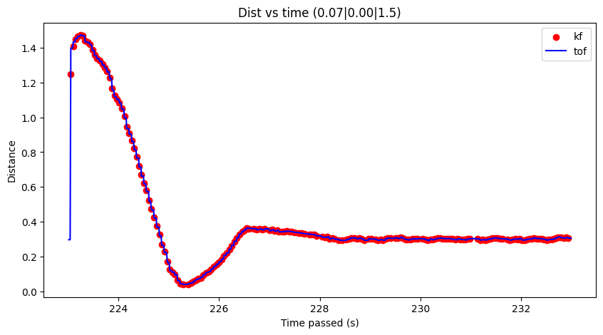
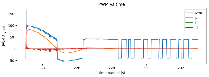
Here are some of my results from running the Kalman Filter! Note that I had to perform some tuning to my sigma values (decreased the sigma_3 to be 5) in order to get improved results; otherwise I received data like in Figure 11.
Result 1
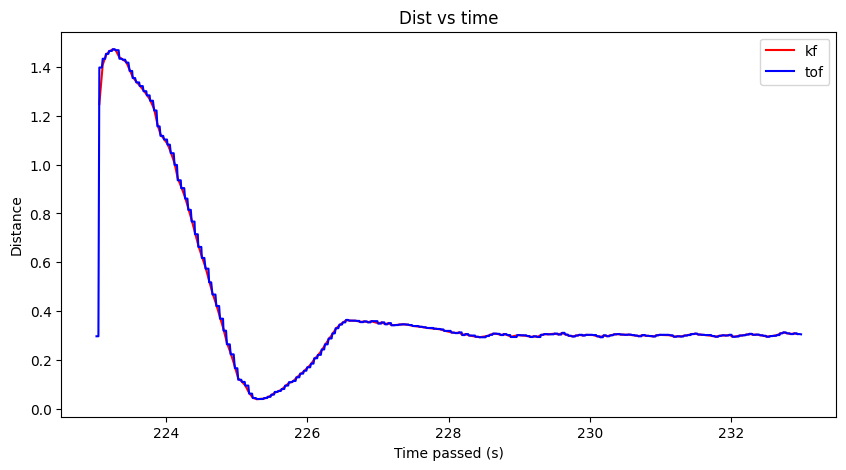
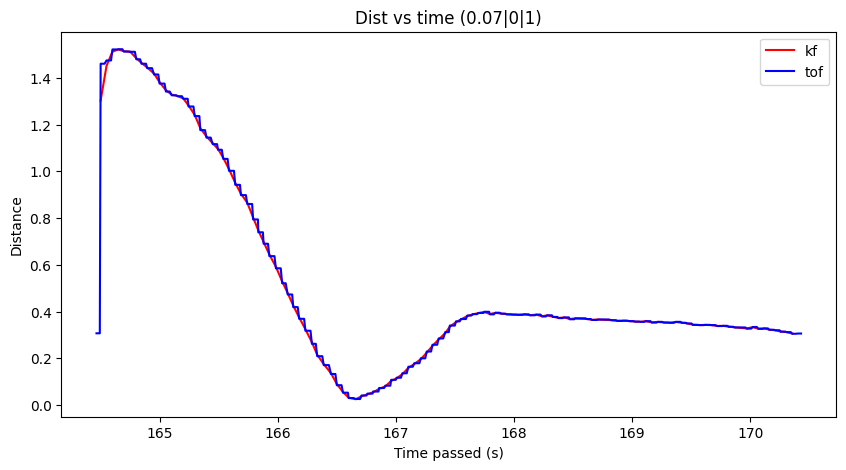
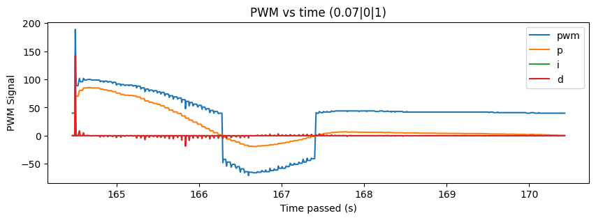
Result 2
Reflection
Overall, I learned a lot about how Kalman Filtering works by implementing it on my robot. I also continued to learn about PID tuning and implementing the Derivative term in PID control.
I think I definitely could have spent more time tuning my PID parameters better, but I didn't get too much time to work on that as implementing the Kalman filter properly took quite some time. I hope to improve my parameter tuning soon though!